SHAP Values Explained: How to Interpret Results and Plots

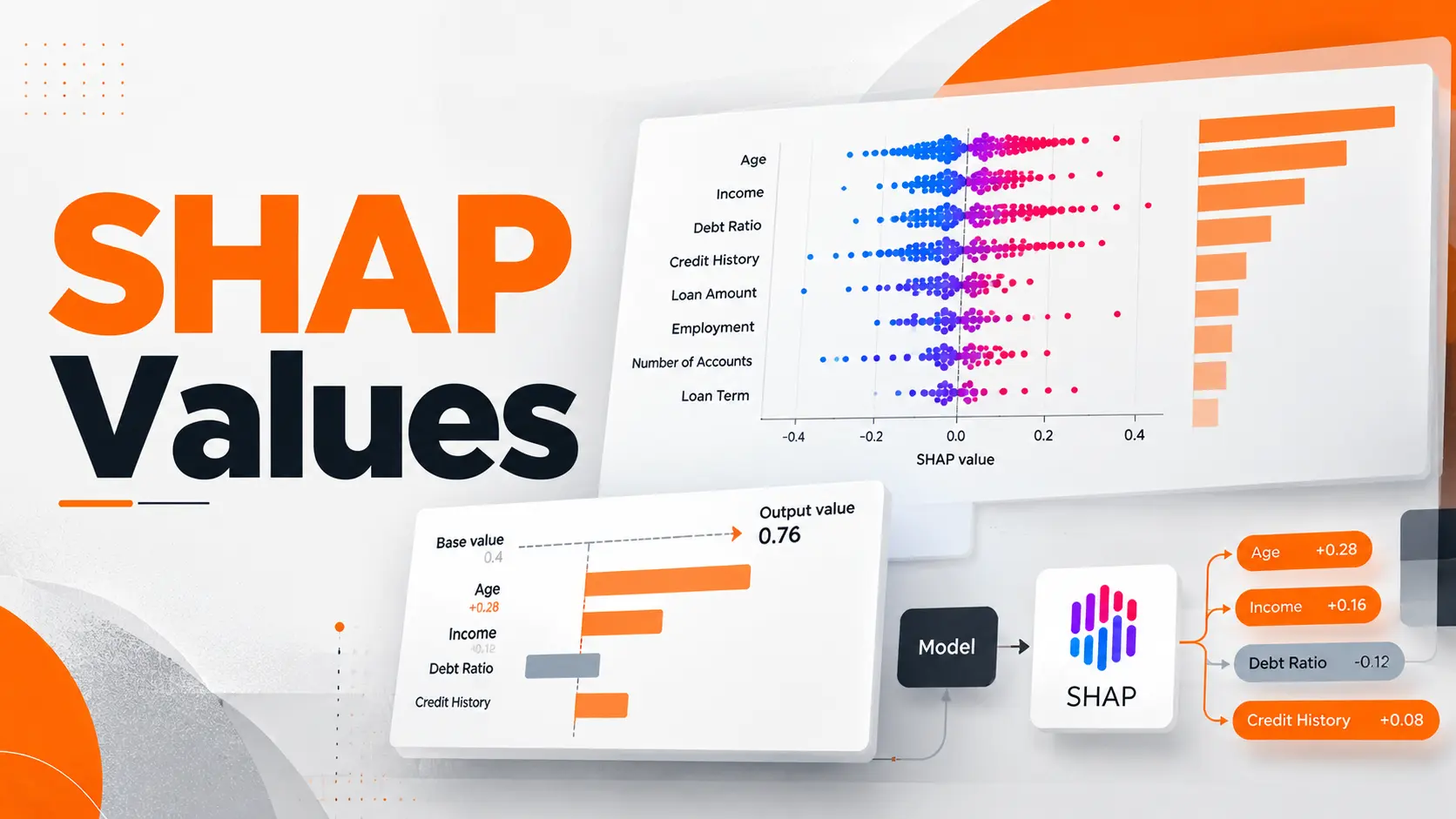
A machine learning model predicts that a house is worth $370,000. The number is clear, but the reasoning behind it is not. SHAP values help explain that prediction by showing how individual features move the model's output above or below a reference value. A positive SHAP value increases the explained output, while a negative value decreases it.

This is one of the most practical applications of Explainable AI. Instead of treating a prediction as a final answer, SHAP gives developers and analysts a way to examine what contributed to it. The important part is understanding those contributions correctly, particularly when reading SHAP plots or explaining decisions to people who did not build the model.

Interpreting SHAP Values

Every SHAP explanation starts with a reference prediction called the base value. Individual features then contribute positive or negative amounts that add up to the model's prediction.

The sign tells you the direction of the contribution. Its magnitude tells you how strongly the feature contributed to that particular prediction, in the units of the output being explained.

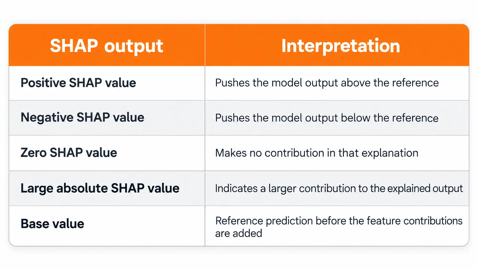
Reference prediction before the feature contributions are added

I start by checking which output the explanation represents. A SHAP value of +0.20 means something different for a model predicting house prices, a model producing probabilities, and a classifier explained in log odds.

It is also important to distinguish a positive contribution from a positive outcome. If the model predicts financial risk, a positive SHAP value can increase the predicted risk. It does not automatically indicate something beneficial.

SHAP Base Value and Prediction Example

A simple numerical example makes SHAP analysis easier to understand.

Consider a property valuation model that estimates house prices using floor area, location, and building age. Suppose its SHAP explanation produces the following values for one property.

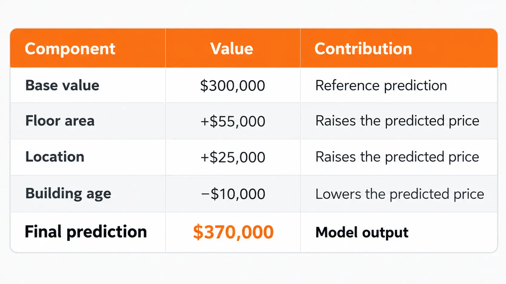
These are illustrative numbers, not the results of a trained property valuation model.

The calculation is straightforward:

$300,000 + $55,000 + $25,000 − $10,000 = $370,000

The base value represents the expected model output under the explainer's reference distribution. The feature contributions explain how the model moves from that starting point to the individual prediction.

In this example, floor area makes the largest positive contribution. Location raises the estimate further, while building age reduces it.

One detail matters here: a negative contribution from building age does not establish that making the building newer would increase its market value by exactly $10,000.

SHAP describes the prediction made by the model. It does not establish a causal relationship between the input and the real world outcome.

How SHAP Values Work

SHAP stands for Shapley Additive Explanations. Its mathematical foundation comes from Shapley values in cooperative game theory.

In game theory, Shapley values distribute the result of cooperation among participating players according to their contributions.

SHAP adapts that idea to machine learning.

The players are the input features, and the result being distributed is the difference between the prediction and its reference value.

A feature's SHAP value reflects its contribution averaged across possible feature combinations under the selected explanation framework.

For an additive SHAP explanation, the central relationship is:

Model prediction = Base value + Sum of SHAP values

This relationship is essential when checking whether an explanation matches the output being examined.

There is another detail worth understanding. The calculation depends on how the explainer represents missing or unavailable features and which reference data or assumptions it uses.

Two explanation configurations can assign different contributions to the same model prediction, particularly when features are correlated.

That does not mean either explanation can be interpreted without context. The explanation method and its assumptions are part of the result.

SHAP Plots and Their Interpretation

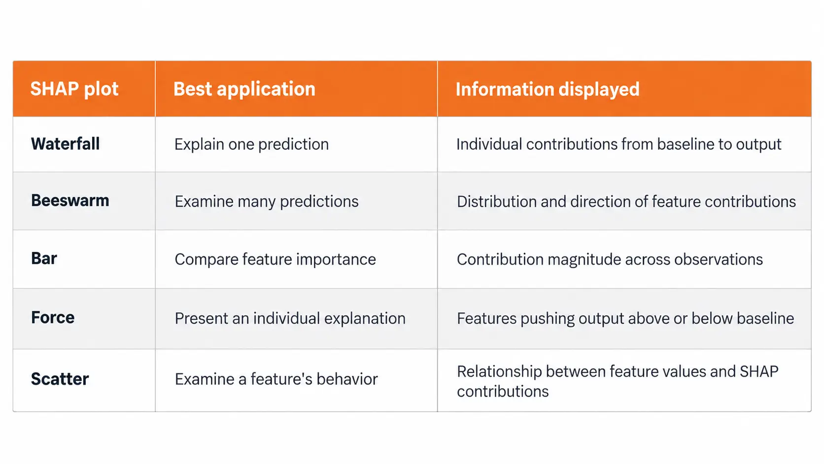
SHAP provides several visualizations for examining feature contributions. Each plot answers a different question, so reading the right chart matters as much as calculating the values.

SHAP Waterfall Plot

A waterfall plot explains one prediction from its base value to its final output.

The chart begins with the reference prediction. Each feature then moves the output upward or downward until the model's prediction is reached.

In the standard SHAP visualization, red bars represent positive contributions and blue bars represent negative contributions.

For the property valuation example, the plot would start at $300,000. Floor area would add $55,000, location would add $25,000, and building age would subtract $10,000.

The final position would be $370,000.

When reading a waterfall plot, I focus on the starting value, the features with the largest contributions, and the final prediction. Those three elements explain most of the information a reader needs.

The waterfall plot is especially useful when investigating one customer record, one financial prediction, or one unusual model output.

SHAP Beeswarm Plot

A beeswarm plot moves from a single prediction to a collection of predictions.

Each dot represents one observation's SHAP value for a feature. Its horizontal position shows the contribution, while its color represents the original feature value when that information is available.

In the standard visualization, red indicates a higher feature value and blue indicates a lower one.

The important distinction is that dot color represents the feature value, not whether the SHAP contribution is positive or negative.

For example, imagine a beeswarm plot where high debt values appear mostly on the positive side of a financial risk model.

That pattern indicates that higher debt values contribute to higher predicted risk for the displayed observations.

If the dots extend widely in both directions, the feature has different contributions across observations.

This plot is useful for understanding variation across a dataset rather than explaining one decision.

SHAP Bar Plot and Feature Importance

A SHAP bar plot can summarize feature importance across many predictions.

For a global summary, features are commonly ranked by their mean absolute SHAP values.

This calculation considers the size of each contribution without allowing positive and negative values to cancel each other.

A feature with a high mean absolute SHAP value has a substantial average contribution to the model outputs over the evaluated observations.

It does not establish that increasing the feature consistently increases the prediction.

SHAP Force and Dependence Plots

Force plots provide another visualization of how features push an individual prediction away from its reference value.

Dependence plots, represented in the current SHAP plotting interface through scatter plots, show how a feature's SHAP contribution varies with its actual value.

A scatter plot can also help reveal variation associated with interactions between features.

The right chart depends on whether the goal is to investigate one prediction, compare observations, or understand broader feature behavior.

Local and Global SHAP Analysis

A useful way to organize SHAP results is to separate local explanations from global analysis.

Local SHAP analysis focuses on one observation.

For a loan application, it identifies the contributions assigned to the applicant's input features. A different applicant can receive a different distribution of SHAP values even when the model uses the same features.

Global SHAP analysis examines explanations across multiple observations.

It helps a team identify features with substantial contributions across its evaluation dataset and investigate whether the model behaves differently across relevant groups.

The distinction matters for product teams.

A customer asking about an individual decision needs a local explanation. A data science team investigating model behavior across thousands of decisions needs a global view.

Neither perspective replaces the other.

SHAP Values for Classification Models

SHAP interpretation becomes more demanding when the model predicts classes or probabilities.

The first step is identifying the model output and the class being explained.

A binary classifier might predict the probability of default, the probability of approval, or a raw score that is transformed into a probability.

These outputs are not interchangeable.

Probability and Log Odds

Consider a binary classifier whose raw output is expressed in log odds.

A base value of zero log odds corresponds to a probability of 50%.

If the combined SHAP contributions increase the raw output by 1, the final log odds become 1, corresponding to a probability of approximately 73.1%.

The change is not one percentage point, and it is not a direct 100 percentage point increase.

The SHAP contributions are additive in log odds, while probabilities are obtained through a nonlinear transformation.

This is particularly important when working with tree models such as XGBoost, where the default raw output for binary classification can be expressed in log odds.

Some explainer configurations support probability outputs directly. In those cases, the contributions must be interpreted in the corresponding probability scale.Before presenting any SHAP chart to business stakeholders, I would confirm the target class, output units, base value, and explainer configuration.

Without those details, even a visually correct SHAP plot can be misunderstood.

Applying SHAP Values to Model Predictions

SHAP analysis begins with a trained machine learning model and a set of predictions that need explanation. The goal is to identify which input features contributed to each result and how strongly they influenced the model's output.

Consider a financial technology company using a model to predict loan repayment risk. The model evaluates information such as income, existing debt, and payment history. SHAP analysis helps the team examine how these features contribute to an individual risk prediction.

The analysis follows three stages:

1. Select the predictions: Identify the model outputs that require explanation, including individual decisions or a representative collection of predictions.

2. Examine feature contributions: Review how each input moves the prediction away from its reference value.

3. Validate the explanation: Confirm that the feature contributions reconstruct the model's output and that the results are interpreted using the correct units.

For a practical assessment, I would compare explanations across applicants with different financial profiles rather than relying on a single prediction. This helps reveal whether the model responds consistently to relevant financial characteristics.

The value of SHAP is not simply identifying influential features. It is providing measurable evidence of how a model uses information, allowing teams to investigate unexpected predictions before relying on them in business decisions.

SHAP Feature Importance and Model Behavior

SHAP feature importance provides a useful summary, but it should not be confused with every other measure of feature importance.

A Random Forest model can provide impurity based feature importance. Permutation analysis measures changes in model performance after disrupting a feature.

SHAP addresses a different question: how features contribute to model outputs under the explanation method's assumptions.

These measures do not have to produce identical rankings.

Consider a model containing two highly correlated features, such as annual income and monthly income.

Both features contain overlapping information. Their attributed contributions can depend on the background distribution and the approach used to account for feature dependence.

A small SHAP contribution does not necessarily mean that the underlying information is irrelevant to the predictive task.

It can mean that the information is also represented by another feature.

For reliable interpretation, feature attribution should be examined alongside knowledge of the dataset and the model's behavior.

Limits of SHAP Interpretation

SHAP explains how a model uses information. It does not establish whether that information is accurate, fair, or appropriate for the decision.

This distinction matters when companies use machine learning in lending, pricing, healthcare, or customer evaluation.

Several aspects deserve attention before interpreting results.

Reference population: SHAP contributions are relative to a baseline. A reference population that does not represent the intended application can produce explanations that are difficult to interpret correctly.

Feature dependence: Correlated inputs create ambiguity in how contributions are distributed. The interpretation depends on the explanation framework and its assumptions.

Model reliability: A detailed explanation does not demonstrate that the underlying prediction is accurate.

Causal meaning: A positive or negative SHAP contribution describes model behavior. It does not prove that changing an input will cause the predicted real world outcome to change.

Dataset coverage: Global conclusions apply to the observations being analyzed. A dataset that excludes important groups cannot establish how explanations behave for those missing groups.

I would treat SHAP as evidence about a model, not as evidence that the model itself is suitable for deployment.

Its greatest practical value comes from connecting feature contributions with model validation, domain knowledge, and the actual decisions the product supports.

Using SHAP Results in AI Products

For an AI startup, SHAP becomes useful when its output leads to a concrete product or engineering decision.

Consider a subscription platform predicting customer cancellations.

Its data science team discovers that one input feature has a large SHAP contribution for several customers identified as high risk.

The next step is not to assume that changing the feature will automatically improve retention.

The team should investigate whether the feature reflects reliable customer behavior, whether it introduces unwanted bias, and whether the prediction remains accurate on representative data.

A local explanation can support investigation of a particular customer prediction. A global analysis can help identify patterns that deserve further testing.

In customer facing products, the explanation should be translated into language appropriate for the audience without presenting statistical associations as verified causes.

The technical chart and the explanation shown to a customer do not need to be identical.

They do need to communicate the model's behavior accurately.

Final Perspective

SHAP values turn a machine learning prediction into a set of measurable feature contributions.

The key to reading them correctly is understanding the base value, the direction and magnitude of each contribution, and the units of the model output.

Waterfall plots explain individual predictions, beeswarm plots reveal patterns across observations, and global summaries help identify influential features.

For developers and product teams, these explanations become valuable when they support investigation and validation rather than simply making a model look transparent.

SHAP can explain how a model arrived at a prediction. Deciding whether that prediction is reliable still requires evidence beyond the explanation itself.

FAQ

Can I use SHAP if I only have access to a model's API?

Yes, provided the API exposes the predictions required by the selected explanation method. Model agnostic approaches can estimate feature contributions through repeated prediction requests. The cost depends on the number of features, reference observations, and API calls. Access permissions and rate limits must be considered.

Why did my SHAP values change after retraining the same model?

Retraining can change the learned relationships and predictions, even when the model architecture remains unchanged. Changes to training records, random seeds, preprocessing, or the explanation baseline can also affect attributions. Meaningful comparisons require documented model versions and consistent explanation settings.

Can I save SHAP explanations for future audits?

Yes. Store the explanation together with the model version, input snapshot, output, explainer configuration, and reference data identifier. Access controls and retention requirements should be applied because explanations and associated inputs can contain sensitive information.

Does SHAP work when my dataset has missing values?

SHAP can explain models that support missing inputs, but the result depends on how missingness is represented and processed. The explanation must reflect the same preprocessing and missing value handling used during prediction. Missing values should not be silently replaced with unrelated defaults solely to make an explainer run.

Can I use SHAP to explain a large language model?

SHAP provides approaches for text models, including token level attribution. However, the computational requirements and interpretation differ from those of tabular prediction models. Token contributions do not establish a complete account of a language model's internal reasoning or prove that generated statements are factually correct.