Prefill vs Decode in LLMs: Key Differences and Performance

Prefill vs Decode describes the two stages of large language model inference. Prefill processes the input prompt in parallel and builds the KV cache, while Decode generates the response one token at a time using that stored information. Prefill places substantial demands on GPU computing capacity, whereas Decode is frequently limited by memory bandwidth.

This distinction explains why an LLM can take several seconds to produce its first token but generate the rest of its response quickly, or begin responding immediately and then stream tokens slowly. Understanding which stage causes the delay is the foundation of effective performance optimization.

Prefill vs Decode: The Performance Difference

The clearest way to understand the difference is to follow a request through both stages.

Consider an LLM receiving a prompt containing 2,000 input tokens and producing a response of 200 output tokens.

During Prefill, the model processes the input sequence and calculates the attention information needed to begin generation. The first output token becomes available after this initial processing.

During Decode, the model generates the remaining output tokens sequentially, using the information calculated during Prefill and the tokens generated so far.

These stages create different performance requirements.

A longer prompt increases the amount of initial processing. A longer response increases the number of sequential generation steps.

The distinction matters because optimizing one stage does not guarantee an improvement in the other.

For a document analysis application processing thousands of input tokens and producing a short summary, prompt processing can represent a substantial share of response time.

For a code generation application producing hundreds of output tokens, sequential decoding can account for most of the total inference time.

The input and output token counts therefore provide the first indication of where execution costs are concentrated.

Prefill: Parallel Prompt Processing

Prefill is the stage in which the model processes the input context before beginning its autoregressive generation loop.

The input can include system instructions, conversation history, retrieved documents, and the latest user message.

Instead of processing each prompt token through a separate generation step, the model performs operations across the input sequence in parallel.

Within the attention mechanism, tokens calculate representations that allow each position to attend to the preceding context according to the model's causal attention rules.

This work produces the Key and Value tensors used during subsequent generation.

Prefill Computation and Context Length

The amount of work required during Prefill depends on the number of input tokens and the model architecture.

Longer prompts increase the number of token representations that must be processed.

For conventional dense attention, the attention calculations include a component whose computational complexity grows quadratically with sequence length.

Other operations, including the model's feedforward layers, have different scaling characteristics.

As a result, doubling the number of prompt tokens does not imply that total Prefill execution time will always double or quadruple.

The actual increase depends on the balance of attention computation, matrix operations, kernel efficiency, and hardware utilization.

In workloads with sufficiently large uncached prompts, Prefill can use the GPU's parallel computing capabilities efficiently.

This is why it is commonly described as a compute bound stage.

Prefix Reuse During Prefill

Not every request requires the model to process its entire prompt from scratch.

When the serving engine supports prefix caching, it can reuse previously calculated Key and Value tensors for a valid matching prompt prefix.

Consider an application sending the same system instructions and reference material with different user questions.

If the shared prefix is available in the cache, the model can process the new portion of the prompt without recalculating the entire shared context.

This reduces the amount of initial computation.

The benefit depends on the actual cache match and the execution engine's caching behavior.

A request containing 10,000 total input tokens can require substantially less Prefill work if most of those tokens already have reusable cached representations.

Therefore, total prompt length and uncached prompt length are not always the same performance measurement.

Decode: Sequential Token Generation

Decode begins after the initial prompt processing has produced the information needed for generation.

The model selects an output token and uses the resulting context to calculate the next one.

Each new token depends on the preceding sequence, so ordinary autoregressive decoding progresses sequentially.

This makes Decode fundamentally different from the parallel processing of the original prompt.

KV Cache During Decode

The KV cache stores attention representations calculated for previous tokens.

During each generation step, the model reads the relevant cached information and calculates the representations required for the new token.

The new Key and Value tensors are then added to the cache.

For conventional full attention, cache storage grows as the sequence becomes longer.

This allows the model to avoid recalculating earlier Key and Value projections, but it also increases the amount of attention information retained in memory.

The model must continue accessing that information as it produces subsequent tokens.

For long contexts, this creates significant memory traffic.

Decode Memory Bandwidth

Autoregressive decoding processes a limited number of new token positions during each iteration.

With small batches, these operations provide less parallel work than processing an entire input prompt.

The GPU repeatedly accesses model weights and cached attention tensors to calculate additional tokens.

When the amount of data being transferred is large relative to the computation performed, memory bandwidth limits execution speed.

This is why Decode is commonly described as a memory bound stage.

The distinction is not absolute.

Larger batches, speculative decoding, model architecture, and attention implementation can increase computational intensity and change the limiting resource.

A reliable performance analysis must consider the actual workload rather than assuming that every Decode operation is limited by memory bandwidth.

GPU Compute and Memory Bandwidth

The difference between Prefill and Decode becomes clearer when examining how efficiently each stage uses GPU hardware.

A GPU has two relevant performance limits: the rate at which it performs mathematical operations and the rate at which it transfers data through memory.

The relationship between these quantities is described by arithmetic intensity.

Arithmetic Intensity = Computational Operations ÷ Bytes Transferred

Operations that perform substantial computation for each byte accessed place greater demands on processing capacity.

Operations that transfer large amounts of data relative to their computation place greater demands on memory bandwidth.

Prefill processes many prompt positions together, creating large matrix operations that can achieve high arithmetic intensity.

Decode operates on fewer new positions at each step and repeatedly accesses weights and KV cache information.

Consequently, the two stages occupy different regions of the GPU performance profile.

The Effect of Batch Size

Batch size changes the amount of work the GPU performs during each execution step.

With one active request, Decode has limited parallel work available.

When several requests decode together, their computations can be batched, allowing more useful work to be performed during a shared execution iteration.

This increases arithmetic intensity and improves hardware utilization under suitable conditions.

However, larger batches also consume more memory and can increase the time required for an individual decoding iteration.

The balance between throughput and latency remains important.

Long Contexts and Attention Costs

Context length also affects the two stages differently.

During Prefill, attention processes relationships among tokens in the input sequence.

During Decode, each newly generated token attends to the retained context.

For conventional full attention, the attention work for one Decode step grows with the number of retained tokens, while the corresponding attention component of a full Prefill grows quadratically with input length.

These relationships explain why long contexts create substantial costs in both stages, even though the underlying performance limitations differ.

Architectures using sliding window attention, compressed attention representations, or other specialized mechanisms change these scaling characteristics.

Prefill vs Decode Comparison

The following table summarizes the differences that matter when evaluating an inference workload.

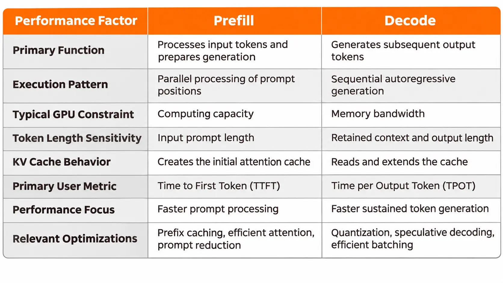
The table describes common behavior rather than fixed hardware rules.

A short uncached Prefill with a very large cached prefix can be limited by memory access. Similarly, Decode with substantial batching can place greater demands on computing capacity.

The useful distinction is how each stage processes tokens and which resources constrain that processing under the measured workload.

TTFT, TPOT, and Inference Latency

Two metrics capture the user experience across Prefill and Decode.

Time to First Token (TTFT) measures the interval between submitting a request and receiving the first generated token.

Time per Output Token (TPOT) measures the average interval between subsequent output tokens after the first.

These measurements describe different parts of response generation.

Understanding TTFT

TTFT reflects more than Prefill computation.

A request can spend time in the network, wait in an execution queue, undergo tokenization, and then enter the Prefill stage.

All these activities contribute to the time the user waits before receiving the first token.

Therefore, high TTFT does not prove that Prefill itself is slow.

Consider two requests with identical prompts.

The first request enters execution immediately. The second waits behind several active requests.

Even if both require the same GPU computation, the second request will have a higher TTFT because of queueing.

Separating queue waiting time from actual Prefill execution time is essential for diagnosis.

Understanding TPOT

TPOT describes the average pace of output generation after the first token.

For a streaming response, it provides a useful measure of how quickly new content appears.

If token generation slows under concurrency, TPOT increases.

However, an average can conceal uneven delivery.

For example, a response might generate several tokens quickly and then pause while the scheduler handles another request.

The average TPOT may remain acceptable even though the interruption affects the user's experience.

For applications that require consistent streaming, individual Inter Token Latency measurements and their upper percentiles provide additional information.

Practical Latency Calculation

Consider an illustrative request with these measured results:

Input tokens: 2,000

Output tokens: 200

TTFT: 600 milliseconds

Average TPOT: 35 milliseconds

The first output token arrives after 600 milliseconds.

The remaining 199 tokens require approximately 6.97 seconds at an average interval of 35 milliseconds.

The total response time is therefore approximately 7.57 seconds.

This example demonstrates why an application can have acceptable initial responsiveness while still taking several seconds to complete its answer.

The reverse can also happen.

A request can spend several seconds waiting or processing a long prompt, then generate a short response in a fraction of that time.

End to end latency alone does not reveal which stage is responsible.

Identifying Prefill and Decode Bottlenecks

The first step in performance diagnosis is to separate application latency from model execution latency.

A useful inference trace should record request arrival, queue admission, Prefill execution, first token generation, subsequent token intervals, and request completion.

This distinction is central to LLM Inference Optimization because improving Prefill and Decode requires different approaches to GPU computation, memory usage, and request scheduling. Identifying the limiting stage helps direct optimization efforts toward the part of inference that actually needs improvement.

The objective is to identify the part of the execution path consuming the largest share of time.

Diagnosing Slow Prefill

When TTFT increases, begin by checking queue waiting time.

If requests spend significant time waiting before GPU execution, the immediate problem is scheduling or available capacity.

If queueing remains low but Prefill execution time increases with uncached input length, prompt processing deserves attention.

Record the number of input tokens, the number of cached tokens, and the duration of Prefill execution.

Compare those measurements across requests using the same model and hardware.

This reveals whether the delay is associated with input processing or another component of the serving system.

Diagnosing Slow Decode

When the first token arrives promptly but the response streams slowly, examine Decode execution.

Measure TPOT, active sequence count, GPU memory usage, and the size of retained contexts.

A model can experience slower decoding as the number of active requests increases.

Longer contexts also increase the amount of attention information accessed during generation.

GPU profiling helps distinguish memory transfer limitations from scheduling overhead and inefficient execution kernels.

If Decode time rises without a corresponding increase in memory traffic or computational work, the serving engine's scheduling behavior deserves closer examination.

Separating Workload Effects

The input and output distribution must remain consistent when comparing results.

A benchmark using short prompts and long responses cannot be compared directly with another using long prompts and short responses.

The two workloads place different demands on Prefill and Decode.

For an informative diagnosis, compare requests with similar input lengths, output lengths, cache states, and concurrency levels.

This prevents workload differences from being mistaken for improvements or regressions in the inference engine.

Prefill Optimization Techniques

Once Prefill has been identified as the limiting stage, optimization should focus on reducing the amount of prompt processing or improving the efficiency of that computation.

Efficient Attention Kernels

Optimized attention implementations such as FlashAttention reduce unnecessary data movement during attention computation.

They improve memory access efficiency and make better use of GPU resources when processing large attention workloads.

The performance benefit depends on context length, model architecture, hardware, and the kernels already used by the serving engine.

Before replacing an attention implementation, confirm whether the runtime already provides an optimized kernel.

Prompt Length and Prefix Caching

Reducing unnecessary input tokens directly reduces the amount of prompt data requiring processing.

For retrieval applications, this means selecting relevant context rather than sending every available document to the model.

The reduction must preserve the information necessary for an accurate response.

Prefix caching provides another improvement when requests share identical reusable prompt prefixes.

Rather than processing the same system instructions or document prefix repeatedly, the serving engine reuses previously calculated attention representations.

The amount of work avoided depends on the length of the valid cached prefix.

Decode Optimization Techniques

Decode optimization focuses on reducing the cost of repeated generation steps and improving the amount of useful work performed by the GPU.

Model Quantization

Quantization reduces the precision of selected model weights and activations.

This can decrease memory consumption and reduce the amount of data transferred during generation.

However, compression alone does not guarantee faster execution.

The improvement depends on hardware support, numerical representation, execution kernels, and quantization overhead.

A quantized configuration should be evaluated using actual Decode latency and model quality measurements.

Speculative Decoding

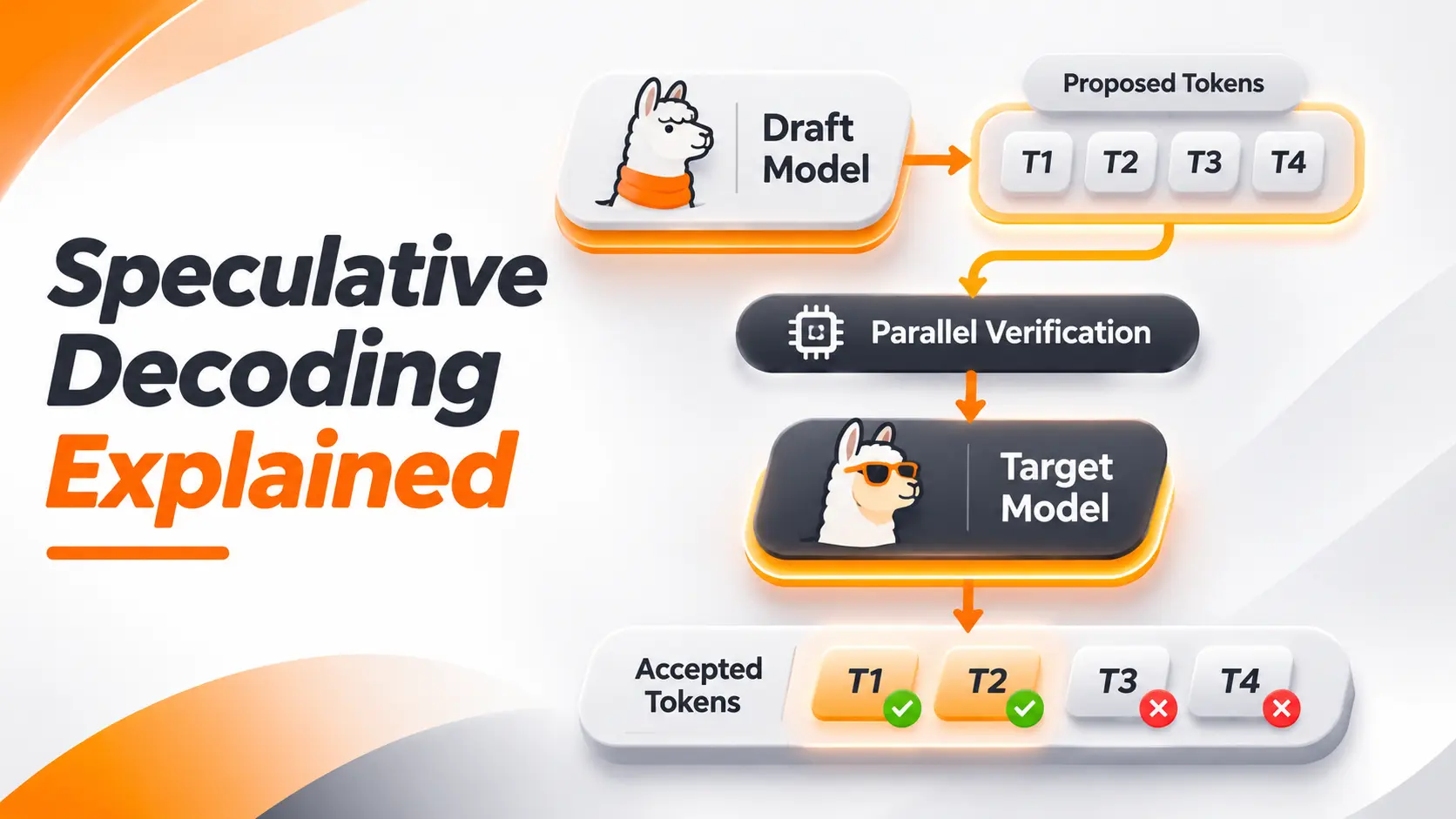
Speculative decoding uses a faster drafting mechanism to propose several output tokens that the target model verifies together.

When sufficient proposals are accepted, the model can advance through multiple token positions without executing the target model separately for every accepted token.

This reduces sequential generation overhead under favorable conditions.

The effectiveness depends on proposal quality, draft computation cost, and verification efficiency.

Its value should be established through measured Decode speed rather than assumed from the number of proposed tokens.

Efficient Batching

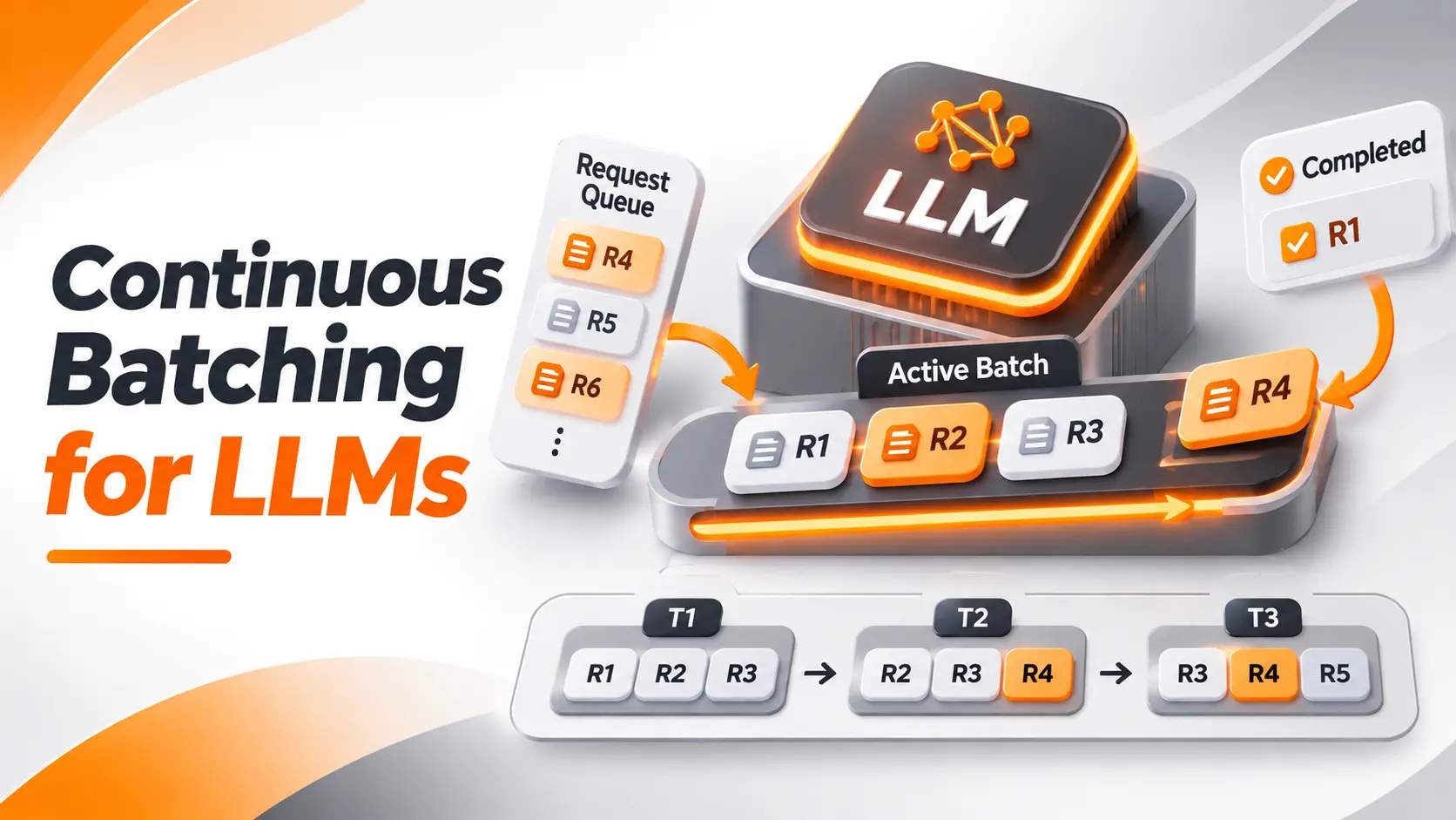
Batching allows multiple active requests to share model execution.

Continuous batching updates the active workload as requests finish, allowing new requests to enter when resources become available.

This improves GPU utilization and aggregate processing capacity.

The tradeoff is competition for computing resources and KV cache memory.

A larger active batch can improve total throughput while increasing the time required to generate individual tokens.

For interactive applications, the configuration must satisfy both throughput and TPOT requirements.

Shared GPU Scheduling and Disaggregated Serving

Prefill and Decode frequently execute on the same GPU.

This creates resource competition because their computational demands differ.

A long Prefill operation can occupy resources needed by requests already generating tokens.

The result can be interruptions in token delivery or increased latency during concurrent traffic.

Chunked Prefill

Chunked Prefill divides a large prompt processing operation into smaller segments.

The scheduler can then interleave those segments with ongoing Decode work.

This provides greater control over how GPU resources are shared between new requests and active generations.

For example, vLLM supports a scheduling budget that limits how many tokens can be processed during an iteration.

A smaller budget can protect Decode responsiveness, while a larger budget can allow more Prefill work to proceed.

The correct setting depends on the traffic pattern and latency requirements.

Prefill Decode Disaggregation

Disaggregated serving assigns Prefill and Decode to separate GPU workers or groups of workers.

This allows the infrastructure to allocate computing resources independently to the two stages.

Prefill workers can focus on prompt processing, while Decode workers are configured for sustained token generation.

However, the KV cache created during Prefill must be made available to the Decode worker.

Transferring that state introduces communication overhead and additional system complexity.

Disaggregation becomes valuable when reduced interference and independent scaling provide benefits greater than the cost of transferring cache data and maintaining separate serving resources.

It is not an automatic improvement for every model or traffic level.

Measuring Performance in Production

A production benchmark should reproduce the application's actual request patterns rather than rely on isolated synthetic prompts.

The dataset should include representative input lengths, output lengths, and concurrent traffic.

It should also record whether requests use reusable cached prefixes.

Start by measuring the existing configuration. Record queue waiting time, Prefill execution time, TTFT, TPOT, throughput, and GPU memory usage.

After making an optimization, repeat the workload under equivalent conditions.

Compare the results separately for short prompts, long prompts, short generations, and extended generations.

This makes it possible to determine whether a change improved the intended stage or merely shifted resource pressure to another part of the system.

Latency and Throughput Tradeoffs

A configuration that improves TTFT can increase TPOT when new prompt processing consumes resources previously available for active decoding.

Similarly, increasing Decode concurrency can improve aggregate throughput while increasing the latency experienced by individual requests.

The correct configuration is determined by the application's performance requirements.

An interactive assistant benefits from a responsive first token and consistent output delivery.

An offline document processing system can prioritize total completion capacity over individual streaming latency.

The measurement should match the service objective rather than optimize a single metric in isolation.

Final Thoughts

Prefill and Decode perform different jobs within the same inference request. Prefill processes the input context and prepares the attention state, while Decode uses that state to generate the response sequentially.

Their performance constraints explain why improving prompt processing does not automatically accelerate output generation.

The practical approach is to measure queueing, Prefill execution, and Decode latency separately before changing the serving configuration.

The most effective optimization targets the stage consuming the resources or time that matters most to the application, while preserving the latency and throughput requirements of the complete system.

FAQ

Does streaming make Prefill or Decode faster?

No. Streaming changes how generated output is delivered to the client. It allows the application to display tokens as they become available but does not inherently accelerate Prefill or Decode computation. Network buffering and client rendering can still affect how quickly the output becomes visible.

Why is my first request slower after starting the model?

The initial request can include additional startup costs such as loading model weights, initializing GPU resources, preparing execution kernels, or completing runtime compilation. These costs are separate from the normal Prefill and Decode work of an established inference session. Maintaining a warm runtime can reduce startup delays at the cost of keeping resources allocated.

Does stopping a response early save inference resources?

Yes. Stopping generation after the request has begun reduces the remaining Decode computation and prevents the KV cache from growing through additional generated tokens. It does not recover the computation already spent processing the original prompt. The saving also depends on how quickly the serving system processes the cancellation.

Can we measure TPOT when the API doesn't stream tokens?

Not directly from a single completed response timestamp. Measuring TPOT requires token generation timestamps or equivalent server metrics. When an API returns only the completed response, the client can measure total latency but cannot isolate token generation intervals accurately without additional telemetry.

Do images and audio inputs go through Prefill too?

Multimodal models process nontext inputs through modality specific components, such as image encoders or audio processing modules, before or alongside language model computation. Their representations can contribute to the language model's input processing workload. The exact division between encoding, Prefill, and Decode depends on the model architecture, so multimodal inference needs separate timing measurements for its additional processing stages.