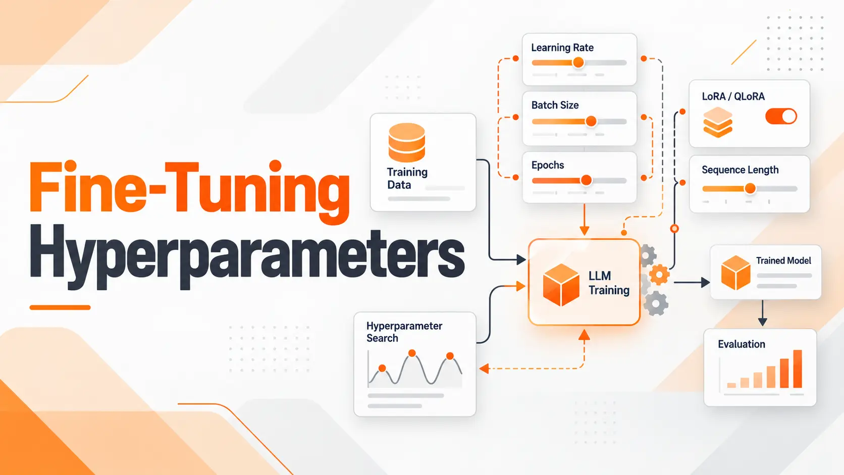
Fine-Tuning Hyperparameters: Settings and Optimization Guide for LLMs

Fine-tuning hyperparameters determine how quickly a language model learns, how many training examples contribute to each update, and how much computational memory the process requires. Learning rate, batch size, and training epochs have the most direct influence on the initial training configuration, but their values must work together.

When working with AI Model Fine-Tuning, I prefer to establish a reliable starting configuration before changing individual settings. The goal is not to achieve the lowest possible training loss. It is to improve the model's performance on unseen requests while keeping the training process stable and resource-efficient.

Fine-Tuning Hyperparameter Starting Settings

The first decision is whether to update the entire model or train a smaller set of adapter parameters through LoRA or QLoRA. These methods require different learning rates and memory configurations.

The following settings provide a practical baseline for supervised fine-tuning of pretrained language models. They are starting values for controlled experiments, not guaranteed optimal settings for every model or dataset.

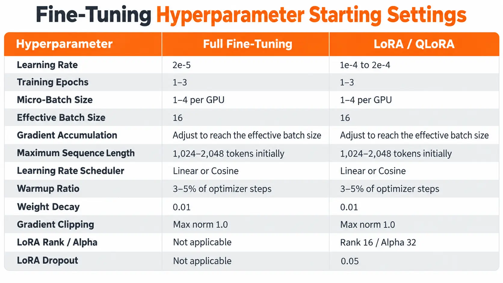
For QLoRA, the adapter settings can remain the same as LoRA while the frozen base model uses 4-bit quantization. NF4 quantization and BF16 computation on compatible hardware provide a memory-efficient training configuration.

I treat this table as the first experiment rather than the final configuration. The model architecture, dataset length, available GPU memory, and validation results determine which values should change.

Learning Rate and Training Stability

Learning rate controls the size of the parameter updates performed by the optimizer. It is one of the most influential fine-tuning hyperparameters because it directly affects how the model moves away from its pretrained weights.

A learning rate that is too high can cause unstable optimization, large loss fluctuations, and deterioration in previously learned capabilities. A rate that is too low can produce limited improvement within the available training steps.

For full-parameter fine-tuning, I use 2e-5 as a conservative starting point. This limits the size of updates across the model's pretrained parameters.

For LoRA training, 1e-4 provides a useful initial setting, with 2e-4 as another value worth evaluating. Adapter training supports higher learning rates because the pretrained base weights remain frozen while the newly introduced adapter parameters are optimized.

I compare these values using the same training examples, effective batch size, evaluation dataset, and training duration.

A learning rate should not be judged by how quickly training loss decreases. The stronger configuration is the one that improves the intended task on held-out examples without causing unacceptable deterioration elsewhere.

Batch Size and Gradient Accumulation

Batch size determines how many examples contribute to an optimization update. It also affects GPU memory consumption and the number of optimizer steps completed during training.

An important distinction exists between micro-batch size and effective batch size.

Micro-batch size is the number of examples processed together on one GPU during a forward and backward pass.

Effective batch size includes the gradients accumulated across multiple micro-batches and all participating GPUs before the optimizer updates the model.

The calculation is:

Effective Batch Size = Micro-Batch Size × Gradient Accumulation Steps × Number of GPUs

Consider a training configuration with a micro-batch size of 2, gradient accumulation set to 8, and one GPU.

The effective batch size is:

2 × 8 × 1 = 16 examples

The model processes eight micro-batches before completing one optimizer update.

This allows training with a larger effective batch without loading all 16 examples into GPU memory simultaneously.

For a dataset containing 2,400 examples, two training epochs and an effective batch size of 16 produce approximately 300 optimizer steps, assuming no examples are dropped and no additional update limits are applied.

I calculate the effective batch size before setting the learning rate schedule. Changing gradient accumulation changes the number of optimizer updates per epoch, even when the number of training examples remains unchanged.

Training Epochs and Early Stopping

An epoch represents one complete pass through the training dataset.

More epochs expose the model to the same examples repeatedly, but additional training does not guarantee better performance on unseen data.

I begin with one to three epochs and evaluate the model at regular intervals. The final epoch count depends on the point at which validation performance reaches its strongest acceptable result.

For a small instruction dataset, repeated exposure can encourage the model to reproduce training examples without developing reliable behavior on new requests.

For a larger and more diverse dataset, the model receives a broader range of examples during each epoch. The number of optimizer updates also changes with dataset size and effective batch size.

This is why comparing epoch counts between unrelated training projects provides limited information.

Selecting the Best Training Checkpoint

The final checkpoint is not automatically the best checkpoint.

I preserve evaluation checkpoints during training and compare their performance on the target task.

If training loss continues decreasing while validation performance deteriorates, additional training is no longer improving generalization according to that evaluation.

Early stopping allows training to end when the monitored validation metric stops improving under the configured stopping rule.

Checkpoint selection should reflect application performance rather than training duration alone.

Learning Rate Schedulers and Warmup

A learning rate scheduler controls how the learning rate changes during training.

Instead of maintaining the same rate throughout the run, the optimizer follows a schedule that adjusts the update size over time.

Two useful starting choices are linear decay and cosine decay.

Linear decay reduces the learning rate at a constant rate after warmup.

Cosine decay follows a curved reduction, maintaining a different learning-rate trajectory during the middle and final stages of training.

Both approaches support controlled fine-tuning. Their relative performance must be evaluated under the same training conditions.

Warmup Steps

Warmup gradually increases the learning rate at the beginning of training rather than applying the configured peak rate immediately.

For an initial experiment, I set warmup to 3–5% of the total optimizer steps.

Using the earlier example of 300 optimizer steps, a 5% warmup requires 15 warmup steps.

I calculate warmup after determining the effective batch size and total training steps. Otherwise, changing batch settings can unintentionally change the fraction of training devoted to warmup.

Weight Decay and Gradient Clipping

Weight decay introduces regularization into the optimization process. With AdamW, it provides decoupled weight decay that can help control the growth of trainable weights.

A starting value of 0.01 gives me a baseline for evaluating whether additional regularization improves validation performance.

Gradient clipping serves a different purpose. Setting the maximum gradient norm to 1.0 limits excessively large gradient updates, helping control optimization instability.

Neither setting compensates for incorrect training targets, unsuitable learning rates, or an unrepresentative evaluation dataset.

LoRA and QLoRA Hyperparameters

LoRA introduces trainable low-rank matrices while preserving the pretrained base weights. This reduces the number of parameters updated during fine-tuning.

Beyond the standard training settings, LoRA introduces three important hyperparameters.

LoRA Rank

Rank, represented by r, determines the dimensions of the low-rank adapter matrices and therefore influences the adapter's trainable parameter count.

A rank of 16 offers a practical baseline for a first experiment.

Increasing rank gives the adapter more capacity to represent parameter updates, but it also increases the number of trainable parameters and their memory requirements.

I increase rank only after evaluating whether the current adapter capacity is limiting task performance.

LoRA Alpha

LoRA Alpha controls the scaling of the adapter updates.

With standard LoRA scaling, the adapter contribution is multiplied by the ratio of Alpha to Rank.

For example, Rank 16 with Alpha 32 produces a scaling factor of 2.

This relationship changes when using Rank-Stabilized LoRA, which scales by Alpha divided by the square root of Rank.

I keep the scaling method fixed while comparing rank configurations. Otherwise, changing rank can also change the effective strength of the adapter updates.

LoRA Dropout and Target Modules

LoRA Dropout applies regularization to adapter training. A value of 0.05 is a reasonable initial setting for a controlled experiment.

Target Modules determine which model layers receive adapters.

Applying adapters to attention projections trains a smaller selection of modules. Targeting all supported linear layers increases coverage and the number of trainable adapter parameters.

The correct choice depends on the architecture and the training objective. For QLoRA-style adaptation, targeting all linear layers is a supported approach.

I confirm the selected modules against the model architecture rather than assuming that parameter names are identical across model families.

Maximum Sequence Length and GPU Memory

Maximum sequence length establishes the number of tokens processed in a training sequence.

This setting affects memory consumption, processing time, and whether complete training examples reach the model.

A sequence length of 1,024 tokens provides an initial configuration for short instruction-response records. Longer conversations or document-processing tasks require enough capacity to preserve the relevant input and target output.

I inspect the token-length distribution of the actual training examples before increasing the limit.

The complete formatted sequence matters, including role markers, system instructions, user content, and target responses.

If the configured maximum length truncates the expected answer, the model cannot learn the complete response from that record.

Reducing GPU Memory Requirements

When training exceeds available GPU memory, I first examine micro-batch size and maximum sequence length.

Reducing the micro-batch size lowers the number of examples held in memory during each pass. Gradient accumulation can preserve the intended effective batch size.

Reducing sequence length lowers memory requirements but can remove necessary training information.

Gradient checkpointing offers another option by recomputing selected activations during backward propagation instead of storing them all.

Mixed-precision training reduces memory requirements and computational costs on compatible hardware. BF16 is a useful option when supported by the GPU and training framework.

For QLoRA, quantizing the frozen base model reduces its weight-storage requirements, although activations, adapter parameters, and optimizer states still consume memory.

The training configuration must fit the hardware without compromising the examples the model needs to learn from.

Hyperparameter Tuning Workflow

I find controlled experiments more useful than changing several settings simultaneously.

A practical tuning process starts with one complete baseline and then investigates the parameters most closely related to the observed performance.

Establishing a Baseline

The baseline includes a fixed model checkpoint, training dataset, validation dataset, random seed, and evaluation procedure.

I record the learning rate, effective batch size, sequence length, optimizer, scheduler, epoch count, and adapter configuration.

This makes later comparisons reproducible and identifies which configuration produced each result.

Comparing Learning Rates

I first compare a small set of learning rates while keeping the remaining settings unchanged.

For LoRA training, a comparison between 5e-5, 1e-4, and 2e-4 provides three distinct learning-rate configurations.

I evaluate the resulting checkpoints using both validation loss and the metric relevant to the application.

For information extraction, that means measuring field-level accuracy or exact matches. For classification, I examine performance across individual categories rather than relying exclusively on overall accuracy.

Refining Training Duration and Batch Size

After identifying a suitable learning-rate configuration, I compare checkpoints from different training stages to select the training duration.

Next, I evaluate changes to effective batch size if training stability, throughput, or available compute makes that necessary.

When effective batch size changes, the number of optimizer steps and learning-rate schedule must be recalculated.

I keep a record of GPU memory usage, training duration, and evaluation performance for every experiment. A configuration that produces a small accuracy improvement at a disproportionately higher computational cost may not be the best choice for deployment.

Training Loss and Validation Results

Training metrics provide evidence about the optimization process, but interpreting them requires more than looking for a downward line.

Training loss declines while validation loss rises. This indicates deterioration in held-out token prediction performance while training fit improves. I inspect training duration, regularization, and data quality before continuing.

Training loss fluctuates sharply. I inspect the learning rate, gradient norms, batch configuration, and numerical precision for instability.

Both training and validation loss remain high. I verify that the training examples contain correct targets, the learning rate allows effective updates, and the selected parameters are actually trainable.

Validation loss improves but task accuracy remains unchanged. I examine the evaluation metric, output formatting, and whether the training objective matches the behavior the application needs.

One detail matters especially in Supervised Fine-Tuning: the loss may be calculated over completion tokens, assistant messages, or the complete sequence, depending on the trainer configuration.

I verify loss masking before interpreting results. Changing which tokens contribute to the loss can make numerical comparisons between training runs misleading.

The same principle applies when comparing datasets with different sequence lengths or target-response structures.

Final Model Selection

Hyperparameter optimization should end with a model selection decision, not simply the lowest recorded loss.

I compare the strongest checkpoints against the original base model on the same independent evaluation set. I also test previously supported capabilities that the application still requires.

The selected configuration must meet the target quality threshold, operate within available hardware limits, and preserve acceptable performance outside the specialized training task.

I retain the model revision, tokenizer, training configuration, dataset version, and evaluation results alongside the final checkpoint. These records make later retraining and performance comparisons considerably more reliable.

Conclusion

Fine-tuning hyperparameters determine how effectively a language model adapts to new tasks, but no individual setting guarantees a successful training run. Learning rate, effective batch size, and training duration provide the foundation, while schedulers, adapter configuration, and sequence length shape the available optimization and memory budget.

I treat a successful configuration as one that demonstrates better performance on independent examples, remains stable during training, and satisfies the application's computational limits. Controlled comparisons turn hyperparameter tuning from guesswork into a measurable engineering process.

FAQ

Can I use the same hyperparameters when switching to a bigger LLM?

The existing configuration can serve as an experimental reference, but it should not be treated as validated for the larger model. Model architecture, parameter count, memory requirements, and optimization behavior can differ. A new baseline evaluation is necessary before selecting the production configuration.

Why did I get different results with the exact same settings?

Identical hyperparameters do not guarantee identical training results. Random initialization of trainable components, data shuffling, dropout, numerical precision, and nondeterministic GPU operations can influence training. Fixed random seeds and deterministic execution settings improve reproducibility, but complete reproducibility also depends on matching software and hardware environments.

Can I change the learning rate without restarting training?

Yes, a supported training framework can modify the learning rate during a run or after resuming from a checkpoint. The optimizer state and learning-rate scheduler must remain consistent with the intended continuation. Changing the rate mid-training also changes the experimental conditions, so the resulting checkpoint should be evaluated separately.

Do I need to retune everything after adding more training data?

Adding examples changes the dataset size and can alter the distribution of training inputs. This affects the number of optimizer steps per epoch and the learning-rate schedule when training is epoch-based. Recalculate training duration and reevaluate the existing configuration before deciding which hyperparameters require further tuning.

Will QLoRA give me the same results as regular LoRA?

Equivalent results are not guaranteed. QLoRA uses quantized base-model weights during adapter training, while standard LoRA can operate with higher-precision base weights. Quantization can influence computations and optimization behavior. Both methods should be compared using the same dataset, task-specific evaluation metrics, and compatible adapter configurations.